Data: catalogs and formats
Gaia Sky needs to first load data in order to display it. The internal
structure of these data is a scenegraph, which is basically a tree
with nodes. The objects that are displayed in a scene are all nodes in
this scene graph and are organized in a hierarchical manner depending on
their geometrical and spatial relations.
The different types of data are:
Catalog data – usually stars which come from a star catalog, but can be any type of point-data. The data descriptor files are in the data folder, and follow the naming convention of
catalog-[name].json. These descriptors are used in the welcome window to enable the selection of catalogs at startup.Rest of data – planets, orbits, constellations, grids and everything else qualifies for this category. These are also described in JSON files. The main file, with pointers to others, is
data-main.json.
Data belonging to either group will be loaded differently into the Gaia Sky. The sections below describe the data format in detail:
Where are the data files defined?
Gaia Sky implements a very flexible an open data mechanism. The data files to be loaded are defined
in a couple of keys in the global.properties configuration file, which is usually located
in the $GS_CONFIG folder (see folders). The keys are:
data.json.catalog– contains a (colon-separated':'on Linux and macOS, semicolon-separated';'on Windows) list of data files which point to the catalogs to load. These files have thecatalog-[name].jsonformat.data.json.objects– contains a (colon-separated':'on Linux and macOS, semicolon-separated';'on Windows) list of data files which point to the files with the rest of the data. By default, only thedata-main.jsonfile is there.
Additionally, any file with the format autoload-[name].json in the data folder will be automatically parsed and loaded using the default JSON loader, so whenever you want to add a group of data that are always loaded, use this naming convention.
catalog-[name].json example files
Catalog files usually contain some metadata on the catlaog (name, description, version, etc.) and a pointer to the actual data. Below is the file catalog-gd1.json which describes the GD1 stream data.
{
"name": "GD1 stream",
"version": 1,
"type": "catalog-gaia",
"description": "GD1 stream with brighter magnitudes",
"link": "https://arxiv.org/abs/1805.00425",
"size": 368633,
"nobjects": 1365,
"data": [{
    "loader": "gaia.cu9.ari.gaiaorbit.data.JsonLoader",
    "files": [ "data/particles-gd1.json" ]
}]
}
Notice that the data ("data -> files") points to another JSON file, which contains some additional info about how to load the data, and a pointer to the actual data files. Here it is:
{
"objects": [{
    "name": "GD1",
    "position": [0.0, 0.0, 0.0],
    "ct": "Stars",
    "fadeout": [1.0e5, 0.5e8],
    "parent": "Universe",
    "impl": "gaia.cu9.ari.gaiaorbit.scenegraph.StarGroup",
    "cataloginfo": {
        "name": "GD1",
        "description": "GD1 stream with brighter magnitudes for visibility",
        "type": "INTERNAL"
    },
    "provider": "gaia.cu9.ari.gaiaorbit.data.group.STILDataProvider",
    "datafile": "data/catalog/gd1/gd1-bright.vot"
    }]
}
As you can see, the STILDataProvider is the one in charge of loading the GD1 data, which resides in a VOTable file, gd1-bright.vot.
data-main.json example file
{
"data" : [
    {
        "loader": "gaiasky.data.JsonLoader",
        "files": [ "data/planets-normal.json",
                    "data/moons-normal.json",
                    "data/satellites.json",
                    "data/asteroids.json",
                    "data/orbits_planet.json",
                    "data/orbits_moon.json",
                    "data/orbits_asteroid.json",
                    "data/orbits_satellite.json",
                    "data/extra-low.json",
                    "data/locations.json",
                    "data/locations_earth.json",
                    "data/locations_moon.json"]
    },
    {
        "loader": "gaiasky.data.stars.SunLoader",
        "files": [ "" ]
    },
    {
        "loader": "gaiasky.data.constel.ConstellationsLoader",
        "files": [ "data/constel_hip.csv" ]
    },
    {
        "loader": "gaiasky.data.constel.ConstelBoundariesLoader",
        "files": [ "data/boundaries.csv" ]
    }]
}
The data-main.json file contains an array, "data", which is a list of pairs
containing [loader: files] correspondences. Each "loader" contains the classes that will load the list of files under the
corresponding "files" property. The main loader, the JsonLoader, expects JSON files as inputs. Each of these files must have an attribute called "objects", which is an array containing the metadata on the objects to load.
As of version 2.1.0, any descriptor file with the name autoload-[name].json dropped into the data
folder will be loaded by default without need to be referenced from any of the properties.
The JSON format
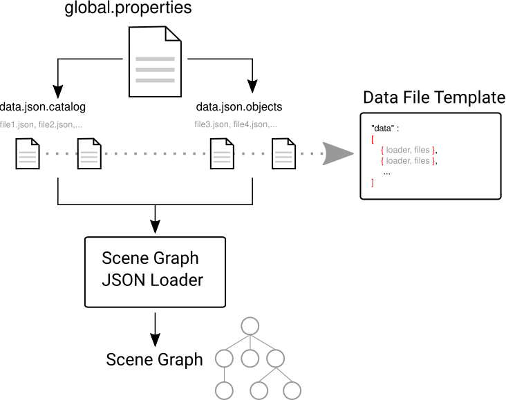
Gaia Sky data loading diagram
The files are sent to the Scene Graph JSON Loader, which iterates on each loader-files pair
in each file, instantiates the loader and uses it to load the files. All loaders need to adhere
to a contract, defined in the interface ISceneGraphLoader (here).
The loadData() method of each loader must return a list of SceneGraphNode objects, which is then
added to a global list containing all the previously loaded files. At the end, we have a list
with all the objects in the scene. This list is passed on to the Scene Graph instance, which
constructs the scene graph tree structure which will contains the object model.
As we said, each loader will load a different kind of data; the
JSONLoader (here)
loads non-catalog data (planets, satellites, orbits, etc.), the STILDataProvider (here) loads VOTables, FITS, CSV and other files through the STIL library, ConstellationsLoader (here) and ConstellationsBoundariesLoader (here) load constellation data and constellation boundary data respectively.
Catalog formats
Catalogs refer to datasets which are essentially particle-based (stars, galaxies, etc.). There are several off-the-shelf options to get catalog data in various formats into Gaia Sky. The most important are VOTable, FITS and CSV. They are all handled by the STIL data provider.
Let’s see an example of the definition of one such catalog in the Oort cloud:
{
    "name" : "Oort cloud",
    "position" : [0.0, 0.0, 0.0],
    "color" : [0.9, 0.9, 0.9, 0.8],
    "size" : 2.0,
    "labelcolor" : [0.3, 0.6, 1.0, 1.0],
    "labelposition" : [0.0484814, 0.0, 0.0484814],
    "ct" : "Others",

    "fadein" : [0.0004, 0.004],
    "fadeout" : [0.1, 15.0],

    "profiledecay" : 1.0,

    "parent" : "Universe",
    "impl" : "gaiasky.scenegraph.ParticleGroup",

    "provider" : "gaiasky.data.group.PointDataProvider",
    "factor" :  149.597871,
    "datafile" : "data/oort/oort_10000particles.dat"
}
Let’s go over the attributes:
name– The name of the particle group.position– The mean cartesian position (see internal reference system) in parsecs, used for sorting purposes and also for positioning the label. If this is not provided, the mean position of all the particles is used.color– The color of the particles as anrgbaarray.size– The size of the particles. In a non HiDPI screen, this is in pixel units. In HiDPI screens, the size will be scaled up to maintain the proportions.labelcolor– The color of the label as anrgbaarray.labelposition– The cartesian position (see internal reference system) of the label, in parsecs.ct– TheComponentType–here–. This is basically astringthat will be matched to the entity type inComponentTypeenum. Valid component types areStars,Planets,Moons,Satellites,Atmospheres,Constellations, etc.fadein– The fade in inetrpolation distances, in parsecs. If this property is defined, there will be a fade-in effect applied to the particle group between the distancefadein[0]and the distancefadein[1].fadeout– The fade out inetrpolation distances, in parsecs. If this property is defined, there will be a fade-in effect applied to the particle group between the distancefadein[0]and the distancefadein[1].profiledecay– This attribute controls how particles are rendered. This is basically the opacity profile decay of each particle, as in(1.0 - dist)^profiledecay, where dist is the distance from the center (center dist is 0, edge dist is 1).parent– The name of the parent object in the scenegraph.impl– The full name of the model class. This should always begaiasky.scenegraph.ParticleGroup.provider– The full name of the data provider class. This must extendgaiasky.data.group.IParticleGroupDataProvider(see here).factor– A factor to be applied to each coordinate of each data point. If not specified, defaults to 1.datafile– The actual file with the data. It must be in a format that the data provider specified inproviderknows how to load.
Star catalogs
Star catalogs are special because, additionally to positional information, they contain extra properties such as proper motions, magnitudes, colors and more. All of these are important to be able to render stars faithfully.
The easiest way to load star catalogs is by loading them from VOTable files. Let’s see how these catalogs can be defined in Gaia Sky. For example, the new Hipparcos reduction:
{
    "name" : "Hipparcos (new red.)",
    "version" : 3,
    "type" : "catalog-star",
    "description" : "Hipparcos new reduction (van Leeuwen, 2007) with curated star names. 117995 stars.",
    "link" : "http://adsabs.harvard.edu/abs/2007ASSL..350.....V",
    "size" : 5433174,
    "nobjects" : 177955,
    "data" : [
    {
        "loader": "gaia.cu9.ari.gaiaorbit.data.JsonLoader",
        "files": [ "data/particles-hip.json" ]
    }]
}
The file particles-hip.json contains a single object with the actual pointer to the VOTable data, and some additional metadata such as the color of labels, a description of the catalog or the data provider:
{
"objects" : [{
            "name" : "Hipparcos (new red.)",
            "position" : [0.0, 0.0, 0.0],
            "color" : [1.0, 1.0, 1.0, 0.25],
            "size" : 6.0,
            "labelcolor" : [1.0, 1.0, 1.0, 1.0],
            "labelposition" : [0.0, -5.0e7, -4.0e8],
            "ct" : "Stars",
            "fadeout" : [21.0e2, 0.5e5],
            "profiledecay" : 1.0,
            "parent" : "Universe",
            "impl" : "gaia.cu9.ari.gaiaorbit.scenegraph.StarGroup",
            "cataloginfo" : {
                    "name" : "Hipparcos",
                    "description" : "Hipparcos new reduction (van Leeuwen, 2007). 117995 stars.",
                    "type" : "INTERNAL"
            },
            "provider" : "gaia.cu9.ari.gaiaorbit.data.group.STILDataProvider",
            "datafile" : "data/catalog/hipparcos/hipparcos.vot"
    }]
}
Regular star catalogs
Gaia Sky supports all formats supported by the STIL library. Since the data held by the formats supported by STIL is not of a unique nature, this catalog loader makes a series of assumptions. More information can be found in STIL data provider.
Particularly, it is possible to directly load a VOTable, CSV, FITS or ASCII file into Gaia Sky using the Open file icon at the bottom of the control panel.
Level-of-detail star catalogs
Gaia Sky uses level-of-detail structures to represent catalogs with hundreds of millions of stars. This broad and deep topic is covered in its own section:
Rest of data
Most of the entities and celestial bodies that are not stars in the Gaia Sky scene are defined in a series of json files and are loaded using the JsonLoader (here).
The format is very flexible and loosely matches the underneath data model, which is a scene graph tree.
Top-level objects
All objects in the json files must have at least the following 5
properties:
name: The name of the object.color: The colour of the object. This will translate to the line colour in orbits, to the colour of the point for planets when they are far away and to the colour of the grid in grids.ct– TheComponentType(here). This is basically astringthat will be matched to the entity type inComponentTypeenum. Valid component types areStars,Planets,Moons,Satellites,Atmospheres,Constellations, etc.impl– The package and class name of the implementing class.parent: The name of the parent entity.
Additionally, different types of entities accept different additional parameters which are matched to the model using reflection. Here are some examples of these parameters:
size– The size of the entity, usually the radius inKm.appmag– The apparent magnitude.absmag– The absolute magnitude.
Below is an example of a simple entity, the equatorial grid:
{
    "name" : "Equatorial grid",
    "color" : [1.0, 0.0, 0.0, 0.5],
    "size" : 1.2e12,
    "ct" : "Equatorial",

    "parent" : "Universe",
    "impl" : "gaiasky.scenegraph.Grid"
}
Planets, moons, asteroids and all rigid bodies
Planets, moons and asteroids all use the model object
Planet (here).
This provides a series of utilities that make their JSON specifications look similar.
Coordinates
Within the coordinates object one specifies how to get the positional data of the entity given a time. This object contains a reference to the implementation class (which must implement IBodyCoordinates here) and the necessary parameters to initialize it. There are currently a bunch of implementations that can be of use:
OrbitLintCoordinates– The coordinates of the object are linearly interpolated using the data of its orbit, which is defined in a separated entity. See the [[Orbits|Non-particle-data-loading#orbits]] section for more info. Thenameof the orbit entity must be given. For instance, the Hygieia moon uses orbit coordinates.
{
    "coordinates" : {
        "impl" : "gaiasky.util.coord.OrbitLintCoordinates",
        "orbitname" : "Hygieia orbit"
    }
}
StaticCoordinates– For entities that never move. A position is required. For instance, the Milky Way object uses static coordinates:
{
    "coordinates" : {
        "impl" : "gaiasky.util.coord.StaticCoordinates",
        "position" : [-2.169e17, -1.257e17, -1.898e16]
    }
}
AbstractVSOP87– Used for the major planets, these coordinates
implement the VSOP87 algorithms. Only the implementation is needed.
For instance, the Earth uses these coordinates.
{
    "coordinates" : {
        "impl" : "gaiasky.util.coord.vsop87.EarthVSOP87"
    }
}
GaiaCoordinates– Special coordinates for Gaia.MoonAACoordinates– Special coordinates for the moon using the algorithm described in the book Astronomical Algorithms by Jean Meeus.
Rotation
The rotation object describes, as you may imagine, the rigid
rotation of the body in question. A rotation is described by the
following parameters:
period– The rotation period in hours.axialtilt– The axial tilt is the angle between the equatorial plane of the body and its orbital plane. In degrees.inclination– The inclination is the angle between the orbital plane and the ecliptic. In degrees.ascendingnode– The ascending node in degrees.meridianangle– The meridian angle in degrees.
For instance, the rotation of Mars:
{
    "rotation": {
        "period" : 24.622962156,
        "axialtilt" : 25.19,
        "inclination" : 1.850,
        "ascendingnode" : 47.68143,
        "meridianangle" : 176.630
    }
}
Model
This object describes the model which must be used to represent the entity. Models can have two origins:
They may come from a 3D model file. In this case, you just need to specify the file.
{
    "model": {
      "args" : [true],
      "model" : "data/models/gaia/gaia.g3db"
    }
}
They may be generated on the fly. In this case, you need to specify the type of model, a series of parameters and the material.
{
    "model": {
      "args" : [true],
      "type" : "sphere",
      "params" : {
        "quality" : 180,
        "diameter" : 1.0,
        "flip" : false
        },
      "material" : {
        "base" : "data/tex/base/earth-day*.jpg",
        "specular" : "data/tex/base/earth-specular*.jpg",
        "normal" : "data/tex/base/earth-normal*.jpg",
        "night" : "data/tex/base/earth-night*.jpg",
        "hieght" : "data/tex/base/earth-height*.jpg",
        "heightScale" : 8.12,
        "reflection" : [ 1.0, 1.0, 0.0 ],
        "elevation" : {
            "noiseType" : "opensimplex",
            "noiseSize" : 10.0,
            "noiseOctaves" : [[1.0, 4.0, 8.0], [1.0, 0.25, 0.125]],
            "noisePower" : 1.0
      }
    }
}
type– the type of model. Possible values aresphere,disc,cylinderandring.params– parameters of the model. This depends on the type. Thequalityis the number of both horizontal and vertical divisions. Thediameteris the diameter of the model andflipindicates whether the normals should be flipped to face outwards. Theringtype also acceptsinnerradiusandouterradius.material– properties of the material, such as textures, reflections, elevation, etc.base– the diffuse texture to use.specular– the specular map to produce specular reflections.normal– normal map to produce extra detail in the lighting.night– texture applied to the part of the model in the shade.height– height map which will be represented with tessellation or parallax mapping (see graphics configuration) and whose scale is defined inheightScale(in Km). It can also contain the keyworkd"generate". In such case, a new subobject"elevation"is expected.noiseType– type of noise. Accepted values areopensimplexandperlin.noiseSize– extent of the noise map to generate.noiseOctaves– a 2xN matrix containing pairs of [frequency, amplitude] for the noise octaves.noisePower– exponent of a power operation on the generated noise (n=n^power).
reflection– specifies an index or a color. If this is present, the default skymap will be used to generate reflections on the surface of the material. Hint: look up theReflectionsobject in Gaia Sky. It is defined insatellites.json.
Atmosphere
Planet atmospheres can also be defined using this object. The
atmosphere object gets a number of physical quantities that are fed
in the atmospheric scattering algorithm (Sean O’Neil, GPU
Gems).
{
    "atmosphere" : {
        "size" : 6600.0,
        "wavelengths" : [0.650, 0.570, 0.475],
        "m_Kr" : 0.0025,
        "m_Km" : 0.001,

        "params" : {
            "quality" : 180,
            "diameter" : 2.0,
            "flip" : true
        }
    }
}
Orbits
When we talk about orbits in this context we talk about orbit lines. In the Gaia Sky orbit lines may be created from two different sources. The sources are used by a class implementing the IOrbitDataProvider (here) interface, which is also specified in their orbit object.
An orbit data file. In this case, the orbit data provider is
OrbitFileDataProvider.The orbital elements, where the orbit data provider is
OrbitalParametersProvider.
If the orbit is sampled it comes from an orbit data file. In the Gaia Sky the orbits of all major planets are sampled, as well as the orbit of Gaia. For instance, the orbit of Venus.
{
    "name" : "Venus orbit",
    "color" : [1.0, 1.0, 1.0, 0.55],
    "ct" : "Orbits",

    "parent" : "Sol",
    "impl" : "gaiasky.scenegraph.Orbit",
    "provider" : "gaiasky.data.orbit.OrbitFileDataProvider",

    "orbit" : {
        "source" : "data/orb.VENUS.dat",
    }
}
If the orbit is defined with its orbital elements, the elements need to be specified in the orbit object. For example, the orbit of Phobos.
{
    "name" : "Phobos orbit",
    "color" : [0.7, 0.7, 1.0, 0.4],
    "ct" : "Orbits",

    "parent" : "Mars",
    "impl" : "gaiasky.scenegraph.Orbit",
    "provider" : "gaiasky.data.orbit.OrbitalParametersProvider",

    "orbit" : {
        "period" : 0.31891023,
        "epoch" : 2455198,
        "semimajoraxis" : 9377.2,
        "eccentricity" : 0.0151,
        "inclination" : 1.082,
        "ascendingnode" : 16.946,
        "argofpericenter" : 157.116,
        "meananomaly" : 241.138
    }
}
Grids and other special objects
There are a last family of objects which do not fall in any of the previous categories. These are grids and other objects such as the Milky Way (inner and outer parts). These objects usually have a special implementation and specific parameters, so they are a good example of how to implement new objects.
{
    "name" : "Galactic grid",
    "color" : [0.3, 0.5, 1.0, 0.5],
    "size" : 1.4e12,
    "ct" : "Galactic",
    "transformName" : "equatorialToGalactic",

    "parent" : "Universe",
    "impl" : "gaiasky.scenegraph.Grid"
}
For example, the grids accept a parameter transformName, which specifies the geometric transform to use. In the case of the galactic grid, we need to use the equatorialToGalactic transform to have the grid correctly positioned in the celestial sphere.
Creating your own catalog loaders
If you want to load your data files into Gaia Sky, chances are that the STIL data provider can already do it.
If you still need to create your own loader, keep reading.
In order to create a loader for your catalog, one only needs to provide an implementation to the ISceneGraphLoader (here) interface.
public interface ISceneGraphLoader {
  public List<? extends SceneGraphNode> loadData() throws FileNotFoundException;
  public void initialize(String[] files) throws RuntimeException;
}
The main method to implement is List<? extends SceneGraphNode> loadData() (here), which must return a list of elements that extend SceneGraphNode.
But how do we know which file to load? You need to create a catalog-*.json file, add your loader there and create the properties you desire. Usually, there is a property called files which contains a list of files to load. Once you’ve done that, implement the initialize(String[]) (here) method knowing that all the properties defined in the catalog-*.json file with your catalogue loader as a prefix will be passed in the Properties p object without prefix.
Also, you will need to connect this new catalog file with the Gaia Sky configuration so that it is loaded at startup. To do so, locate your global.properties file (usually under $GS_CONFIG, see folders) and add your new file to the property data.json.catalog.
Add your implementing jar file to the classpath (usually putting it in the lib/ folder should do the trick) and you are good to go.
Take a look at already implemented catalogue loaders such as the OctreeCatalogLoader (here)
to see how it works.
Loading data using scripts
Data can also be loaded at any time from a Python script. See the scripting section for more info.